Running the Analysis
Source:vignettes/articles/cookbook_running_the_analysis.Rmd
cookbook_running_the_analysis.RmdRunning the Analysis
This section outlines the key steps for running the PACTA for Banks analysis, beginning with a high-level overview followed by a detailed breakdown of each step. Code snippets are provided to ensure a straightforward implementation in your own R environment.
Structure of the Workflow
If you have prepared or obtained all required input datasets as outlined in Preparatory Steps, you can then proceed with the PACTA for Banks analysis through the following main steps:
- Setup: Load the necessary packages and import the data.
- Matching process: Match counterparties in the loan book to companies in the asset-based company data.
- Calculate PACTA metrics: Run the analysis to assess loan book alignment with transition scenario benchmarks.
- Plot PACTA metrics: Generate standard PACTA visualizations to support result interpretation.
Fig. 1: Structure of the Workflow
These steps are generally sequential, but achieving the best possible match rate often requires multiple iterations. The matching process may need to be refined and repeated to improve accuracy. The following sections provide a detailed breakdown of each step.
Setup
We use the pacta.loanbook package for key functions and example datasets. Additionally, we leverage dplyr, readxl, and readr for optional but convenient data manipulation and import functions.
Import Data
We need two datasets to begin, as described in the Preparatory Steps chapter: a loanbook and an asset-based company dataset (abcd). For more detail about the necessary structure of these datasets, see the data dictionaries for loanbook and abcd.
To simulate having these data files prepared, we will use the demo data included in the pacta.loanbook package to create example XLS files using the writexl package.
library(writexl)

writexl::write_xlsx(
  x = loanbook_demo,
  path = file.path(tempdir(), "loanbook.xlsx")
)

writexl::write_xlsx(
  x = abcd_demo,
  path = file.path(tempdir(), "abcd.xlsx")
)
Typically, these data files are stored in XLS files on your computer. As an example, they could be imported as in the code below using the readxl package, however, if you use custom data that does not strictly follow the format as defined in the previous section, you may need to adjust the import code and/or do some data manipulation in R after importing.
loanbook <- readxl::read_excel(path = file.path(tempdir(), "loanbook.xlsx"))

loanbook
#> # A tibble: 283 × 13
#>    id_loan id_direct_loantaker name_direct_loantaker       id_ultimate_parent name_ultimate_parent                   loan_size_outstanding loan_size_outstanding_currency loan_size_credit_limit loan_size_credit_limit_currency sector_classification_system sector_classification_direct_loantaker lei_direct_loantaker isin_direct_loantaker
#>    <chr>   <chr>               <chr>                       <chr>              <chr>                                                  <dbl> <chr>                                           <dbl> <chr>                           <chr>                        <chr>                                  <chr>                <lgl>
#>  1 L1      C294                Vitale Group                UP15               Scholz KGaA                                           225625 EUR                                          18968805 EUR                             NACE                         D35.11                                 NA                   NA
#>  2 L2      C293                Moen-Moen                   UP84               NA                                                    301721 EUR                                          19727961 EUR                             NACE                         D35.11                                 NA                   NA
#>  3 L3      C292                Rowe-Rowe                   UP288              Harvey, Harvey and Harvey                             410297 EUR                                          20811147 EUR                             NACE                         D35.11                                 801600ATB1D513IUFZ77 NA
#>  4 L4      C299                Fadel-Fadel                 UP54               NA                                                    233049 EUR                                          19042869 EUR                             NACE                         D35.11                                 NA                   NA
#>  5 L5      C305                Ring AG & Co. KGaA          UP104              Conti, Conti e Conti SPA                              406585 EUR                                          20774115 EUR                             NACE                         D35.11                                 NA                   NA
#>  6 L6      C304                Kassulke-Kassulke           UP83               Farrell, Farrell and Farrell                          185721 EUR                                          18570711 EUR                             NACE                         D35.11                                 108200TUBGG1DR0QR635 NA
#>  7 L7      C227                Morissette Group            UP134              Weller AG                                             184793 EUR                                          18561453 EUR                             NACE                         D35.11                                 NA                   NA
#>  8 L8      C303                Barone s.r.l.               UP163              Williamsonn PLC                                       291513 EUR                                          19626123 EUR                             NACE                         D35.11                                 NA                   NA
#>  9 L9      C301                Werner Werner AG & Co. KGaA UP138              Leone-Leone s.r.l.                                    407513 EUR                                          20783373 EUR                             NACE                         D35.11                                 NA                   NA
#> 10 L10     C302                De rosa s.r.l.              UP32               Benedetti, Benedetti e Benedetti Group                186649 EUR                                          18579969 EUR                             NACE                         D35.11                                 NA                   NA
#> # ℹ 273 more rows

abcd <- readxl::read_excel(path = file.path(tempdir(), "abcd.xlsx"))

abcd
#> # A tibble: 4,972 × 12
#>    company_id name_company                          lei                  sector technology          production_unit  year production emission_factor plant_location is_ultimate_owner emission_factor_unit
#>    <chr>      <chr>                                 <chr>                <chr>  <chr>               <chr>           <dbl>      <dbl>           <dbl> <chr>          <lgl>             <chr>
#>  1 175        Giordano, Giordano e Giordano e figli 18500033XH6RG332SX89 power  hydrocap            MW               2020    121032.          NA     MY             TRUE              tonnes of CO2 per per hour per MW
#>  2 175        Giordano, Giordano e Giordano e figli 18500033XH6RG332SX89 power  hydrocap            MW               2021    119274.          NA     MY             TRUE              tonnes of CO2 per per hour per MW
#>  3 175        Giordano, Giordano e Giordano e figli 18500033XH6RG332SX89 power  hydrocap            MW               2022    117515.          NA     MY             TRUE              tonnes of CO2 per per hour per MW
#>  4 175        Giordano, Giordano e Giordano e figli 18500033XH6RG332SX89 power  hydrocap            MW               2023    115757.          NA     MY             TRUE              tonnes of CO2 per per hour per MW
#>  5 175        Giordano, Giordano e Giordano e figli 18500033XH6RG332SX89 power  hydrocap            MW               2024    113999.          NA     MY             TRUE              tonnes of CO2 per per hour per MW
#>  6 175        Giordano, Giordano e Giordano e figli 18500033XH6RG332SX89 power  hydrocap            MW               2025    112240.          NA     MY             TRUE              tonnes of CO2 per per hour per MW
#>  7 526        Vitali, Vitali e Vitali s.r.l.        887100CAVZ6Y3KYT3Q90 cement integrated facility tonnes per year  2020   6327858.           0.723 CI             TRUE              tonnes of CO2 per tonne of cement
#>  8 526        Vitali, Vitali e Vitali s.r.l.        887100CAVZ6Y3KYT3Q90 cement integrated facility tonnes per year  2021   6569983.           0.735 CI             TRUE              tonnes of CO2 per tonne of cement
#>  9 526        Vitali, Vitali e Vitali s.r.l.        887100CAVZ6Y3KYT3Q90 cement integrated facility tonnes per year  2022   6812108.           0.746 CI             TRUE              tonnes of CO2 per tonne of cement
#> 10 526        Vitali, Vitali e Vitali s.r.l.        887100CAVZ6Y3KYT3Q90 cement integrated facility tonnes per year  2023   7054232.           0.758 CI             TRUE              tonnes of CO2 per tonne of cement
#> # ℹ 4,962 more rows
Matching Process
The next step after loading all required input files is to run the matching process, where you will match loans from the loanbook data with production data from the ABCD dataset
The matching process is divided into three main steps:
- Apply Matching Algorithm – Calculate match precision scores between the loan book and ABCD datasets.
- Validate Matches – Manually review matches, selecting the correct company when multiple exceed the threshold score.
- Prioritize Matches – Pick validated matches by priority level.
The following sections provide a detailed breakdown of each step.
Apply Matching Algorithm – Calculate match precision scores between the loan book and ABCD datasets
match_name() scores the match between names in a
loanbook dataset and names in an asset-based company dataset. The names
come from the columns name_direct_loantaker and
name_ultimate_parent of the loanbook dataset, and from the
column name_company of the asset-based company dataset. In
the loan book data set, it is possible to optionally add any number of
name_intermediate_parent_* columns, where *
indicates the level up the corporate tree from
direct_loantaker.
The raw names are internally transformed applying best-practices commonly used in name matching algorithms, such as:
- Remove special characters
- Replace language specific characters
- Abbreviate certain names to reduce their importance in the matching
- Remove corporate suffixes when necessary
- Spell out numbers to increase their importance
The similarity is then scored between the internally-transformed
names of the loanbook against the names in the abcd. For more
information on the scoring algorithm used, see
stringdist::stringsim().
The basic usage of match_name() is as follows:
matched <- match_name(loanbook, abcd)

matched
#> # A tibble: 326 × 22
#>    id_loan id_direct_loantaker name_direct_loantaker       id_ultimate_parent name_ultimate_parent         loan_size_outstanding loan_size_outstanding_currency loan_size_credit_limit loan_size_credit_limit_currency sector_classification_system sector_classification_direct_loantaker lei_direct_loantaker isin_direct_loantaker id_2dii level   sector sector_abcd name  name_abcd score source borderline
#>    <chr>   <chr>               <chr>                       <chr>              <chr>                                        <dbl> <chr>                                           <dbl> <chr>                           <chr>                        <chr>                                  <chr>                <lgl>                 <chr>   <chr>   <chr>  <chr>       <chr> <chr>     <dbl> <chr>  <lgl>
#>  1 L1      C294                Vitale Group                UP15               Scholz KGaA                                 225625 EUR                                          18968805 EUR                             NACE                         D35.11                                 NA                   NA                    UP190   ultima… power  power       Scho… Scholz K… 1     loanb… FALSE
#>  2 L3      C292                Rowe-Rowe                   UP288              Harvey, Harvey and Harvey                   410297 EUR                                          20811147 EUR                             NACE                         D35.11                                 801600ATB1D513IUFZ77 NA                    UP101   ultima… power  power       Harv… Harvey, … 1     loanb… FALSE
#>  3 L5      C305                Ring AG & Co. KGaA          UP104              Conti, Conti e Conti SPA                    406585 EUR                                          20774115 EUR                             NACE                         D35.11                                 NA                   NA                    UP39    ultima… power  power       Cont… Conti, C… 1     loanb… FALSE
#>  4 L6      C304                Kassulke-Kassulke           UP83               Farrell, Farrell and Farrell                185721 EUR                                          18570711 EUR                             NACE                         D35.11                                 108200TUBGG1DR0QR635 NA                    DL129   direct… power  power       Kass… Kassulke… 1     loanb… FALSE
#>  5 L6      C304                Kassulke-Kassulke           UP83               Farrell, Farrell and Farrell                185721 EUR                                          18570711 EUR                             NACE                         D35.11                                 108200TUBGG1DR0QR635 NA                    UP63    ultima… power  power       Farr… Farrell,… 1     loanb… FALSE
#>  6 L7      C227                Morissette Group            UP134              Weller AG                                   184793 EUR                                          18561453 EUR                             NACE                         D35.11                                 NA                   NA                    DL179   direct… power  power       Mori… Moretti … 0.911 loanb… FALSE
#>  7 L7      C227                Morissette Group            UP134              Weller AG                                   184793 EUR                                          18561453 EUR                             NACE                         D35.11                                 NA                   NA                    UP224   ultima… power  power       Well… Weller AG 1     loanb… FALSE
#>  8 L8      C303                Barone s.r.l.               UP163              Williamsonn PLC                             291513 EUR                                          19626123 EUR                             NACE                         D35.11                                 NA                   NA                    UP228   ultima… power  power       Will… Williams… 0.987 loanb… FALSE
#>  9 L9      C301                Werner Werner AG & Co. KGaA UP138              Leone-Leone s.r.l.                          407513 EUR                                          20783373 EUR                             NACE                         D35.11                                 NA                   NA                    DL274   direct… power  power       Wern… Wende We… 0.844 loanb… FALSE
#> 10 L9      C301                Werner Werner AG & Co. KGaA UP138              Leone-Leone s.r.l.                          407513 EUR                                          20783373 EUR                             NACE                         D35.11                                 NA                   NA                    UP132   ultima… power  power       Leon… Leone-Le… 1     loanb… FALSE
#> # ℹ 316 more rows
match_name() defaults to scoring matches between name
strings that belong to the same sector. This implies that a potential
match will only be shown if the names in the loanbook and the ABCD are
sufficiently similar AND the loan is classified in the same sector as
the company activity in the ABCD Using by_sector = FALSE
removes this limitation – increasing computation time, and the number of
potentially incorrect matches to manually validate. In most cases, it is
recommended to keep by_sector = TRUE. However, lifting the
restriction can be helpful in cases where the sector classification in
the loanbook is not reliable or no sector classification is available at
all. Below you can see that the removal of the restriction increases the
number of potential matches.
The match_name() function, by default, scores matches
between name strings within the same sector. This means a potential
match is shown only if: - The names in the loan book and ABCD dataset
are sufficiently similar. - The loan is classified in the same sector as
the company activity in the ABCD dataset.
Setting by_sector = FALSE removes this restriction,
which: - Increases computation time. - Increases the number of potential
(but possibly incorrect) matches requiring manual validation.
In most cases, keeping by_sector = TRUE is recommended.
However, disabling the sector restriction can be useful when sector
classifications in the loan book are unreliable or missing. Below, you
can see how removing the restriction increases the number of potential
matches.
match_name(loanbook, abcd, by_sector = FALSE) %>% nrow()
#> [1] 656

# Compare to
match_name(loanbook, abcd, by_sector = TRUE) %>% nrow()
#> [1] 326
The min_score argument sets a minimum threshold score
for matching precision. This helps by: - Filtering out imprecise matches
by setting a higher threshold. - Adding more potential matches if the
default suggestions do not provide enough coverage.
The default value is 0.8, but you can adjust it between 0 and 1. A higher score means stricter matching, resulting in fewer potential matches.
The example below sets the threshold to 0.9:
match_name(loanbook, abcd, min_score = 0.9) %>%
  pull(score) %>%
  range()
#> [1] 0.9007692 1.0000000
Validate Matches – Manually review matches, selecting the correct company when multiple exceed the threshold score
After calculating initial match scores, you must manually review the suggested matches to decide which to keep or remove. This step is critical for ensuring a high quality match result, especially in text-based matching, where similar company names may not actually refer to the same entity.
Manual validation helps to:
- Prevent incorrect matches from affecting the analysis.
- Ensure accuracy in linking loan book data to the ABCD dataset.
- Improve overall match precision, especially when iterating to enhance coverage.
Since this step is not automated, it requires effort, often making it the most time-consuming part of the process.
To begin, save the output of match_name() to a CSV file for review. For example, using readr:
After exporting the match results, you must manually review, edit,
and save the data: - Open the file – Load
matched.csv in a spreadsheet editor (Excel, Google Sheets,
etc.). - Compare matches – Verify if the
name (loan book) and name_abcd (ABCD)
correspond to the same entity. Use additional details (sector, company
structure, internal data) to improve accuracy. - Edit the
data: - If the match is valid, set the score value
to 1. - If the match is incorrect or uncertain, leave the
score as-is or set it to a value other than 1.
- Save the edited file: as
valid_matches.csv.
Once validated, re-import the edited file into R, for example, using readr:
valid_matches <- readr::read_csv(file = file.path(tempdir(), "valid_matches.csv"), show_col_types = FALSE)You can find more detailed information about the matching process under the header “PACTA for Banks Training Webinar 2” in the training materials section of the PACTA for Banks website and in the corresponding slide deck.
Prioritize Matches – Pick validated matches by priority level
The validated dataset may have multiple matches per loan. Consider
the case where a loan is given to “Acme Power USA”, a subsidiary of
“Acme Power Co.”. There may be both “Acme Power USA” and “Acme Power
Co.” in the abcd, and so there could be two valid matches
for this loan. To get the best match only, use prioritize()
– it picks rows where score is 1 and level per
loan is of highest priority:
some_interesting_columns <- c("id_loan", "level", "score")

prioritized_matches <-
  valid_matches %>%
  prioritize()

prioritized_matches %>% select(all_of(some_interesting_columns))
#> # A tibble: 177 × 3
#>    id_loan level            score
#>    <chr>   <chr>            <dbl>
#>  1 L6      direct_loantaker     1
#>  2 L13     direct_loantaker     1
#>  3 L20     direct_loantaker     1
#>  4 L21     direct_loantaker     1
#>  5 L22     direct_loantaker     1
#>  6 L24     direct_loantaker     1
#>  7 L25     direct_loantaker     1
#>  8 L26     direct_loantaker     1
#>  9 L27     direct_loantaker     1
#> 10 L28     direct_loantaker     1
#> # ℹ 167 more rows
By default, highest priority refers to the most granular match
(direct_loantaker). The default priority is set internally
via prioritize_level().
prioritize_level(valid_matches)
#> [1] "direct_loantaker" "ultimate_parent"
You may use a different prioritization stratgey by passing a function
to the priority argument of prioritize().
A Note on Sector Classifications and the borderline
Flag
Sector Classifications
Matches are preferred when the sector from the loanbook
matches the sector from the abcd. The loanbook
sector is determined internally by mapping the sector classification
code from the loan book to a PACTA sector, using the
sector_classification_system and
sector_classification_direct_loantaker columns. Currently,
the following options are supported for
sector_classification_system, specified in
sector_classifications:
GICS, ISIC, NACE, NAICS, PSIC, SIC
The borderline flag
An issue arises when, for example, a company is classified in the
“power transmission” sector. In a perfect world, these companies would
produce no electricity, and we would not try to match them. In practice,
however, we find there is often overlap, as companies may have
integrated business models that span multiple steps of the supply chain
or sector classification systems do not break down every code clearly
enough to map it to PACTA sectors unambiguously. For this reason, we
introduced the borderline flag.
In the example below, we see two classification codes coming from the NACE classification standard:
nace_classification %>%
  filter(code %in% c("D35.11", "D35.14", "D35.1"))
#> # A tibble: 3 × 6
#>   original_code description                      code  sector borderline version
#>   <chr>         <chr>                            <chr> <chr>  <lgl>      <chr>
#> 1 35.1          35.1 Electric power generation,… D35.1 power  TRUE       2.1
#> 2 35.11         35.11 Production of electricity… D35.… power  FALSE      2.1
#> 3 35.14         35.14 Distribution of electrici… D35.… power  TRUE       2.1
Notice that the code D35.11 corresponds to power generation. This is
an identical match to power sector in PACTA, and thus the
borderline flag is set to FALSE. In contrast,
code D35.14 corresponds to the distribution of electricity. In a perfect
world, we would set this code to not in scope, however
there is still a chance that these companies produce electricity. For
this reason, we have mapped it to power with
borderline = TRUE. Finally, code D35.1 corresponds to the
wider electricity sector, covering “Electric power generation,
transmission and distribution”. This is a case where the granularity is
insufficient to unambiguously match the code to the power
sector as defined in PACTA, and thus the borderline flag is
set to TRUE.
In practice, if a company has a sector code with
borderline is TRUE and is matched,
then consider the company in scope. If it has a borderline
value TRUE and is not matched, then consider it
out of scope.
Optional: Prepare own sector classification mapper
If you can obtain sector codes in any one of those classification systems for your loan book, it is strongly recommended using them. If you do not have your loans mapped to any of these systems, you can either run the matching without a sector classification (see above), or you can use a custom sector classification system.
If you want to use your own custom sector classification system, you
will need to create a file that follows the same structure as the sector
classification files in sector_classifications, that is,
the file needs to contain the following columns (of the following
types):
-
sector: <character> -
borderline: <logical> -
code: <character> -
code_system: <character>
Please notice that when manually preparing a custom sector
classification file, you need to decide for every code of your mapping
system which PACTA sector the code maps to. This requires the system to
be relatively granular to capture the nuances of the supply chains of
the companies in your loan book. As discussed above, any sector code
that is not unambiguously in scope or out of scope for a given PACTA
sector should be marked TRUE in the borderline
column. Any sector code that is clearly not in scope should be marked
FALSE and receive the sector value
not in scope. Any sector code that is clearly in scope
should be marked FALSE for borderline and
receive the PACTA sector value that it maps to in the
sector column.
For a code example how to implement your own sector classification system, see the sector classification example in the match_name reference.
Calculate the Match Success Rate
pacta.loanbook allows you to match loans from your loanbook to the companies in an asset-based company dataset. However, not all loans will have a match – some companies may be missing from the ABCD dataset, or they may operate outside the PACTA focus sectors (power, cement, oil and gas, aviation, coal, automotive, steel, and hdv).
To assess how much of your loan book is successfully matched, you can calculate matching coverage in two ways:
By dollar value: Measure the portion of your loan book covered, using one of the
loan_size_*columns.By company count: Count the number of companies matched.
To visualize matching coverage, first load the ggplot2 package:
We will use the example datasets created in the previous section. To
illustrate the point, we create a loanbook dataset with two
mismatched loans:
loanbook <- loanbook %>%
  mutate(
    name_ultimate_parent =
      ifelse(id_loan == "L1", "unmatched company name", name_ultimate_parent),
    sector_classification_direct_loantaker =
      ifelse(id_loan == "L2", "99", sector_classification_direct_loantaker)
  )
We will then run the matching algorithm on this loanbook:
matched <- loanbook %>%
    match_name(abcd) %>%
    prioritize()
#> Warning: Some values in `sector_classification_direct_loantaker` are unknown: "99"
#> ℹ The unknown values do not appear in the specified sector classification
#>   system.
The matched dataset contains only successfully
matched loans. To determine coverage, we need to refer back to the
original loanbook dataset and classify each loan according to the PACTA
sectors using the sector_classification_direct_loantaker
column.
To achieve this, we merge loanbook with the
sector_classifications dataset, which includes all sector
classification standards used by PACTA. However, there are two technical
caveats to consider:
- Column name differences: The datasets use different column names for
sector classifications. We use
dplyr::left_join()with thebyargument to merge:
-
sector_classification_systemandsector_classification_direct_loantaker(fromloanbook) -
code_systemandcode(fromsector_classifications)
- Data type mismatch: The sector classification codes have different
data types in the two datasets. To prevent errors in
dplyr::left_join():
- We convert
sector_classification_direct_loantakerto match the type ofcodebefore merging. - After merging, we restore its original type.
merge_by <- c(
    sector_classification_system = "code_system",
    sector_classification_direct_loantaker = "code"
  )

loanbook_with_sectors <- loanbook %>%
  left_join(sector_classifications, by = merge_by) %>%
  mutate(sector_classification_direct_loantaker = as.character(sector_classification_direct_loantaker))
To generate the coverage dataset, we merge these two
datasets together:
coverage <- left_join(loanbook_with_sectors, matched) %>%
  mutate(
    loan_size_outstanding = as.numeric(loan_size_outstanding),
    loan_size_credit_limit = as.numeric(loan_size_credit_limit),
    matched = case_when(
      score == 1   ~ "Matched",
      is.na(score) ~ "Not Matched",
      TRUE         ~ "Not Matched"
    ),
    sector = case_when(
      borderline == TRUE & matched == "Not Matched" ~ "not in scope",
      TRUE ~ sector
    )
  )
#> Joining with `by = join_by(id_loan, id_direct_loantaker, name_direct_loantaker,
#> id_ultimate_parent, name_ultimate_parent, loan_size_outstanding,
#> loan_size_outstanding_currency, loan_size_credit_limit,
#> loan_size_credit_limit_currency, sector_classification_system,
#> sector_classification_direct_loantaker, lei_direct_loantaker,
#> isin_direct_loantaker, sector, borderline)`
1. Calculate loanbook coverage by dollar value
Using the coverage dataset, we can measure total loan
book coverage based on dollar value. To facilitate this, we define two
helper functions:
- A function to calculate coverage by dollar value.
- A plotting function to visualize coverage.
dollar_value <- function(data, ...) {
  data %>%
    summarize(loan_size_outstanding = sum(loan_size_outstanding), .by = c(matched, ...))
}

plot_coverage <- function(data, x, y) {
  ggplot(data) +
    geom_col(aes({{x}}, {{y}}, fill = matched)) +
    # Use more horizontal space -- avoids overlap on x axis text
    theme(legend.position = "top")
}
Let’s first explore all loans.
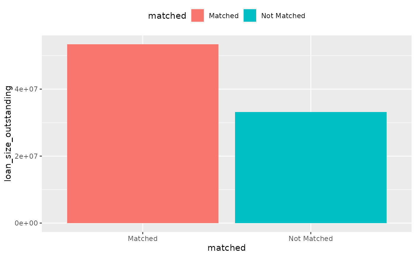
To calculate the total, in-scope, loanbook coverage:
coverage %>%
  filter(sector != "not in scope") %>%
  dollar_value() %>%
  plot_coverage(matched, loan_size_outstanding)
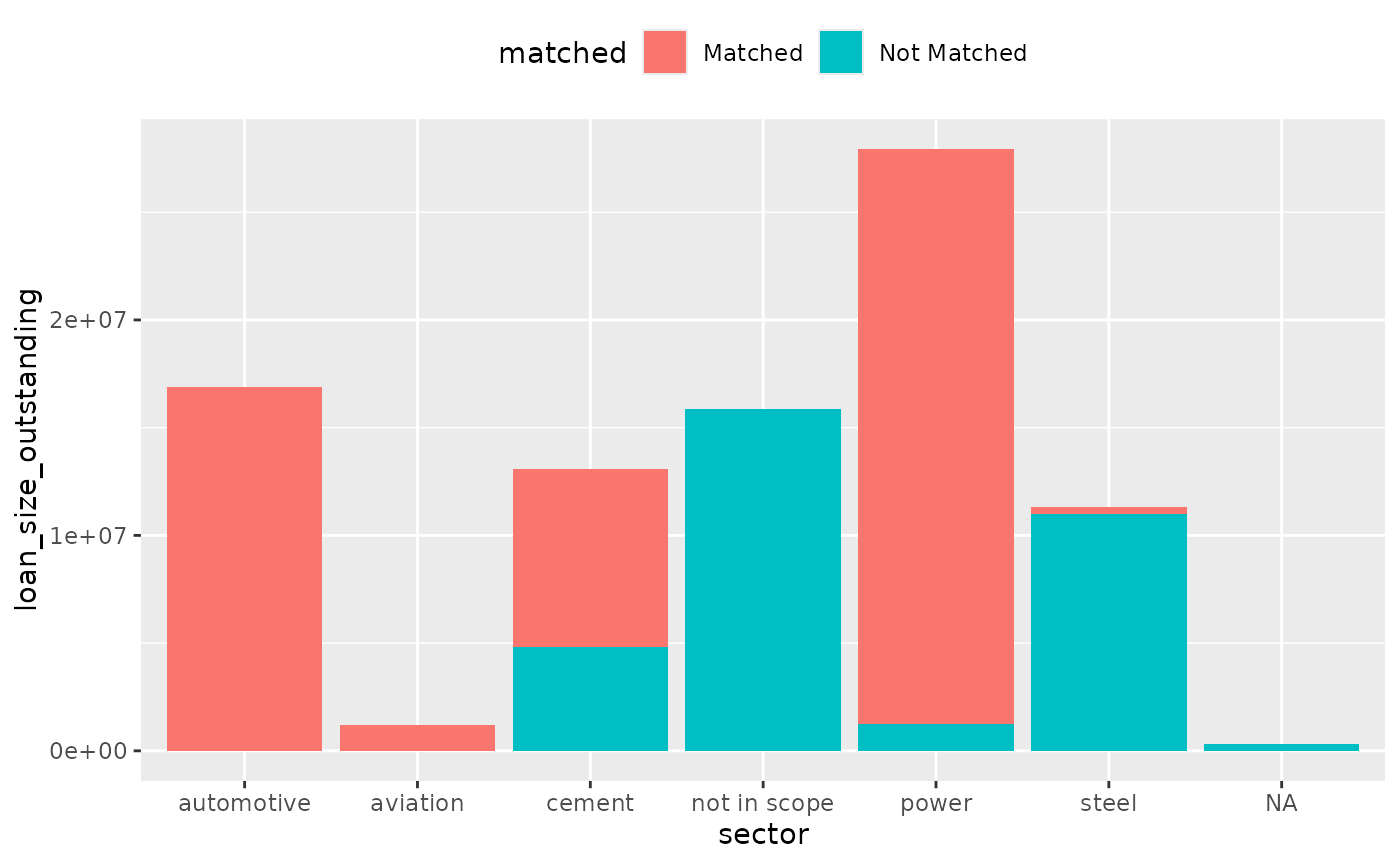
You may break-down the plot by sector:
Or even further, by matching level:
coverage %>%
  mutate(matched = case_when(
    matched == "Matched" & level == "direct_loantaker"      ~ "Matched DL",
    matched == "Matched" & level == "intermediate_parent_1" ~ "Matched IP1",
    matched == "Matched" & level == "ultimate_parent"       ~ "Matched UP",
    matched == "Not Matched"                                ~ "Not Matched",
    TRUE                                                    ~ "Catch unknown"
  )) %>%
  dollar_value(sector) %>%
  plot_coverage(sector, loan_size_outstanding)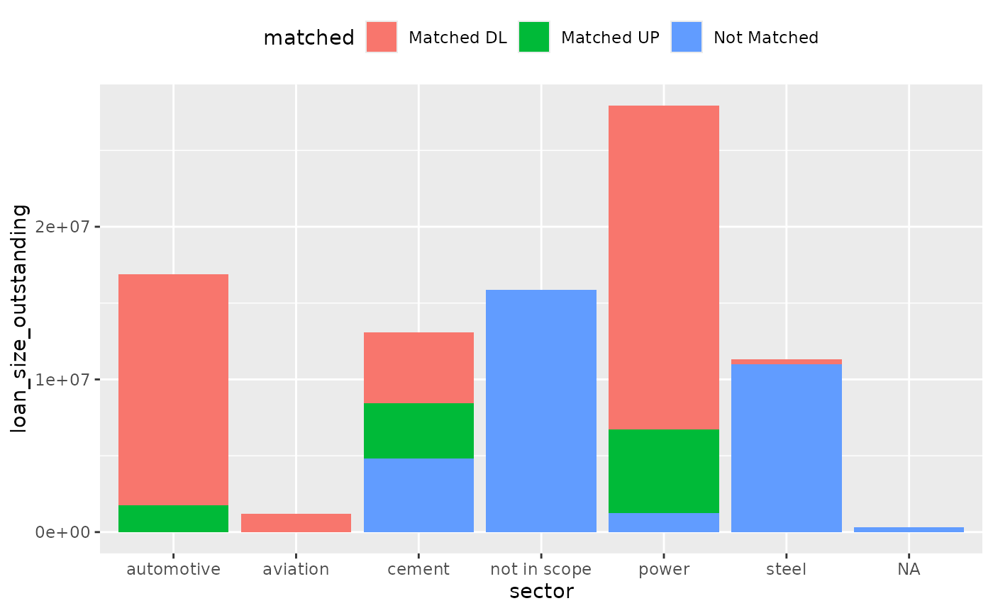
2. Count the number of companies matched
Another useful metric is the number of companies in your loan book
that were successfully matched. The most relevant level for this
analysis is likely the direct_loantaker level.
companies_matched <- coverage %>%
  summarize(no_companies = n_distinct(name_direct_loantaker), .by = c(sector, matched))

companies_matched %>%
  plot_coverage(sector, no_companies)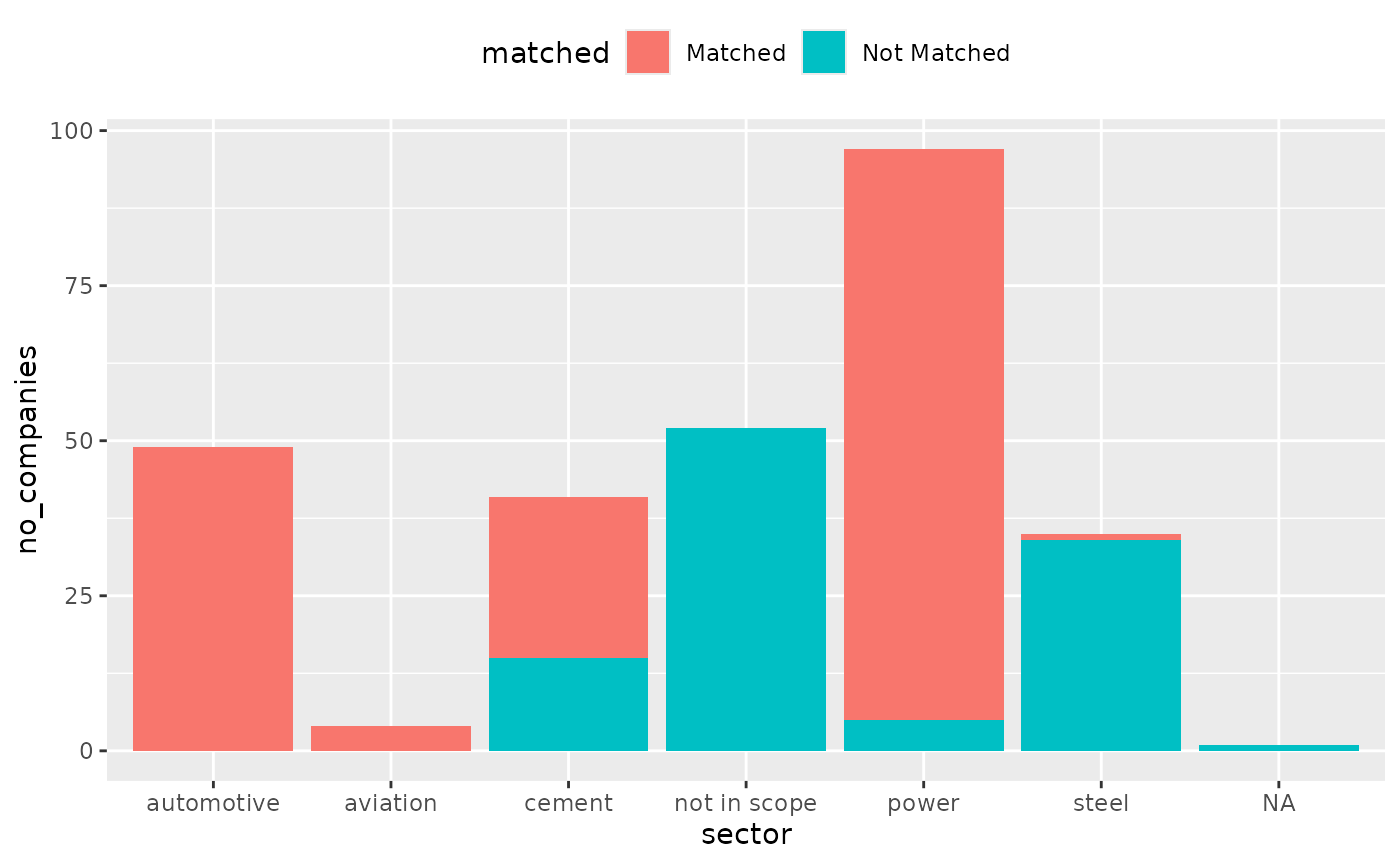
Optional: Handling misclassified loans
A misclassified loan occurs when a counterparty is incorrectly identified as belonging to a PACTA sector based on the sector classification in the loan book.
Why does misclassification matter? - It artificially lowers match success rates by expecting matches that do not exist in the ABCD dataset. - Iterating the matching process will not help—if a company does not operate in an in-scope sector, no adjustments will create a valid match. - A reliable match success rate requires an accurate denominator, meaning only loans truly within an in-scope sector should be included.
Misclassification is typically identified manually by reviewing unmatched counterparties to determine if they should be in scope. Since this process can be time-consuming, it is best to prioritize unmatched loans with the largest credit amounts, as they have the greatest impact on the match success rate.
Since misclassified loans cannot be matched, leaving them in the dataset skews results. While correction is not mandatory, adjusting large misclassified loans is strongly recommended for more accurate analysis.
Options for Handling Misclassified Loans
Once misclassified loans have been identified, there are two options:
- Correct the classification in the loanbook:
- Update the raw loanbook to reflect the correct sector.
- Re-run the matching process to ensure the loan is matched appropriately
- Keep documentation of changes for replicability
- Adjust match success rate calculation:
- If modifying the raw loanbook is not possible, exclude misclassified loans from the success rate calculation.
- Create a
loans_to_remove.csvfile containing a single column,id_loan, listing the misclassified loans. - Remove these loans from the match success calculation to avoid misleading results.
The first option is generally preferred, as it ensures loans are assigned to the correct sector.
Once the list of misclassified loans is identified, there are two broad options to appropriately these cases.
Example
Suppose a loan with ID L255 is falsely classified as a steel company but actually produces steel-based products, making it part of the downstream value chain rather than primary steel production. Since it cannot be matched to ABCD, but the sector classification cannot be changed, we handle it by creating a CSV file with its ID.
This correction process can be done programmatically or manually, ensuring more accurate match success rate reporting.
readr::write_csv(
  x = tibble(id_loan = "L255"),
  file = file.path(tempdir(), "loans_to_remove.csv")
)
The loans_to_remove.csv file should have just one
column, id_loan, and therefore be structured as
follows:
-
id_loan: <character>
We then read in the file and remove the misclassified loan from the match success rate calculation. We compare the coverage before and after the removal of the misclassified loan to see the impact of the correction. For demonstration purposes, we artificially increase the loan_size_outstanding of the affected counterparty while focusing on the steel sector only, to see the clear impact.
coverage_compare <- coverage %>%
  mutate(
    loan_size_outstanding = ifelse(id_loan == "L255", 50000000, loan_size_outstanding)
  ) %>%
  filter(sector == "steel")

coverage_compare %>%
  mutate(matched = case_when(
    matched == "Matched" & level == "direct_loantaker"      ~ "Matched DL",
    matched == "Matched" & level == "intermediate_parent_1" ~ "Matched IP1",
    matched == "Matched" & level == "ultimate_parent"       ~ "Matched UP",
    matched == "Not Matched"                                ~ "Not Matched",
    TRUE                                                    ~ "Catch unknown"
  )) %>%
  dollar_value(sector) %>%
  plot_coverage(sector, loan_size_outstanding)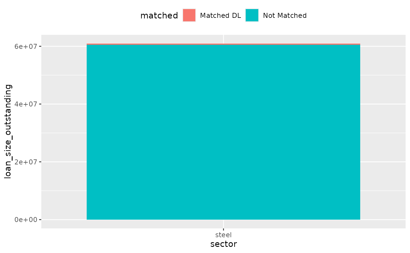
loans_to_remove <- readr::read_csv(file.path(tempdir(), "loans_to_remove.csv"))

coverage_corrected <- coverage_compare %>%
  anti_join(loans_to_remove, by = "id_loan")

coverage_corrected %>%
  mutate(matched = case_when(
    matched == "Matched" & level == "direct_loantaker"      ~ "Matched DL",
    matched == "Matched" & level == "intermediate_parent_1" ~ "Matched IP1",
    matched == "Matched" & level == "ultimate_parent"       ~ "Matched UP",
    matched == "Not Matched"                                ~ "Not Matched",
    TRUE                                                    ~ "Catch unknown"
  )) %>%
  dollar_value(sector) %>%
  plot_coverage(sector, loan_size_outstanding)
Calculate PACTA alignment metrics
PACTA alignment metrics can be calculated using two approaches: the Market Share Approach and the Sectoral Decarbonization Approach. If a sector has a technology-level scenario pathway you can use the Market Share Approach whereas sector-level scenario pathways will use the Sectoral Decarbonization Approach. If you are using the scenarios prepared by RMI, you will have the following pairing of approaches, sectors and technologies:
Market Share Approach
The Market Share Approach sets scenario targets based on the production of a technology within a sector. For example, it can define targets for electric vehicle production in the automotive sector. This approach is recommended for sectors with detailed technology roadmaps.
Targets can be set at the portfolio level:
# Use these datasets to practice but eventually you should use your own data.
scenario <- scenario_demo_2020
regions <- region_isos_demo

market_share_targets_portfolio <-
  target_market_share(
    data = prioritized_matches,
    abcd = abcd,
    scenario = scenario,
    region_isos = regions
  )

market_share_targets_portfolio
#> # A tibble: 1,076 × 10
#>    sector     technology  year region scenario_source metric     production technology_share scope  percentage_of_initial_production_by_scope
#>    <chr>      <chr>      <dbl> <chr>  <chr>           <chr>           <dbl>            <dbl> <chr>                                      <dbl>
#>  1 automotive electric    2020 global demo_2020       projected     145649.            0.165 sector                                  0
#>  2 automotive electric    2020 global demo_2020       target_cps    145649.            0.165 sector                                  0
#>  3 automotive electric    2020 global demo_2020       target_sds    145649.            0.165 sector                                  0
#>  4 automotive electric    2020 global demo_2020       target_sps    145649.            0.165 sector                                  0
#>  5 automotive electric    2021 global demo_2020       projected     147480.            0.165 sector                                  0.000739
#>  6 automotive electric    2021 global demo_2020       target_cps    146915.            0.165 sector                                  0.000511
#>  7 automotive electric    2021 global demo_2020       target_sds    153332.            0.167 sector                                  0.00310
#>  8 automotive electric    2021 global demo_2020       target_sps    147258.            0.165 sector                                  0.000649
#>  9 automotive electric    2022 global demo_2020       projected     149310.            0.165 sector                                  0.00148
#> 10 automotive electric    2022 global demo_2020       target_cps    148155.            0.164 sector                                  0.00101
#> # ℹ 1,066 more rows
or at the company level:
market_share_targets_company <-
  target_market_share(
    data = prioritized_matches,
    abcd = abcd,
    scenario = scenario,
    region_isos = regions,
    by_company = TRUE, # Output results at company-level
    weight_production = FALSE
  )

market_share_targets_company
#> # A tibble: 14,505 × 11
#>    sector     technology  year region scenario_source name_abcd                         metric     production technology_share scope  percentage_of_initial_production_by_scope
#>    <chr>      <chr>      <dbl> <chr>  <chr>           <chr>                             <chr>           <dbl>            <dbl> <chr>                                      <dbl>
#>  1 automotive electric    2020 global demo_2020       Bernardi, Bernardi e Bernardi SPA projected     324592.           0.0759 sector                                         0
#>  2 automotive electric    2020 global demo_2020       Bernardi, Bernardi e Bernardi SPA target_cps    324592.           0.0759 sector                                         0
#>  3 automotive electric    2020 global demo_2020       Bernardi, Bernardi e Bernardi SPA target_sds    324592.           0.0759 sector                                         0
#>  4 automotive electric    2020 global demo_2020       Bernardi, Bernardi e Bernardi SPA target_sps    324592.           0.0759 sector                                         0
#>  5 automotive electric    2020 global demo_2020       Christiansen PLC                  projected     512438.           0.130  sector                                         0
#>  6 automotive electric    2020 global demo_2020       Christiansen PLC                  target_cps    512438.           0.130  sector                                         0
#>  7 automotive electric    2020 global demo_2020       Christiansen PLC                  target_sds    512438.           0.130  sector                                         0
#>  8 automotive electric    2020 global demo_2020       Christiansen PLC                  target_sps    512438.           0.130  sector                                         0
#>  9 automotive electric    2020 global demo_2020       Donati, Donati e Donati s.r.l.    projected     277214.           1      sector                                         0
#> 10 automotive electric    2020 global demo_2020       Donati, Donati e Donati s.r.l.    target_cps    277214.           1      sector                                         0
#> # ℹ 14,495 more rows
These results can be saved/written to a CSV file for potential input to other models and software, for example:
readr::write_csv(x = market_share_targets_portfolio, file = file.path(tempdir(), "market_share_targets_portfolio.csv"))
readr::write_csv(x = market_share_targets_company, file = file.path(tempdir(), "market_share_targets_company.csv"))
Remember to replace tempdir() with the path to the
directory that you wish to save your files in.
Sectoral Decarbonization Approach
The Sectoral Decarbonization Approach sets scenario targets based on a sector’s emission factor. For example, it can define targets for the average emission factor in the cement sector. This approach is recommended for sectors without detailed technology roadmaps.
# Use this dataset to practice but eventually you should use your own data.
co2 <- co2_intensity_scenario_demo

sda_targets_portfolio <-
  target_sda(
    data = prioritized_matches,
    abcd = abcd,
    co2_intensity_scenario = co2,
    region_isos = regions
  ) %>%
  filter(sector == "cement", year >= 2020)
#> Warning: Removing rows in abcd where `emission_factor` is NA

sda_targets_portfolio
#> # A tibble: 110 × 6
#>    sector  year region             scenario_source emission_factor_metric emission_factor_value
#>    <chr>  <dbl> <chr>              <chr>           <chr>                                  <dbl>
#>  1 cement  2020 advanced economies demo_2020       projected                             0.0230
#>  2 cement  2020 developing asia    demo_2020       projected                             0.0595
#>  3 cement  2020 global             demo_2020       projected                             0.664
#>  4 cement  2021 advanced economies demo_2020       projected                             0.0232
#>  5 cement  2021 developing asia    demo_2020       projected                             0.0594
#>  6 cement  2021 global             demo_2020       projected                             0.665
#>  7 cement  2022 advanced economies demo_2020       projected                             0.0233
#>  8 cement  2022 developing asia    demo_2020       projected                             0.0592
#>  9 cement  2022 global             demo_2020       projected                             0.666
#> 10 cement  2023 advanced economies demo_2020       projected                             0.0235
#> # ℹ 100 more rows
or at the company level:
sda_targets_company <-
  target_sda(
    data = prioritized_matches,
    abcd = abcd,
    co2_intensity_scenario = co2,
    region_isos = regions,
    by_company = TRUE # Output results at company-level
  )
#> Warning: Removing rows in abcd where `emission_factor` is NA

sda_targets_company
#> # A tibble: 966 × 7
#>    sector  year region             scenario_source name_abcd                          emission_factor_metric emission_factor_value
#>    <chr>  <dbl> <chr>              <chr>           <chr>                              <chr>                                  <dbl>
#>  1 cement  2020 advanced economies demo_2020       Milani, Milani e Milani SPA        projected                              0.714
#>  2 cement  2020 developing asia    demo_2020       Heidrich GmbH                      projected                              0.675
#>  3 cement  2020 developing asia    demo_2020       Hovel Hovel GmbH & Co. KGaA        projected                              0.622
#>  4 cement  2020 global             demo_2020       Battaglia-Battaglia Group          projected                              0.626
#>  5 cement  2020 global             demo_2020       Bergstrom, Bergstrom and Bergstrom projected                              0.607
#>  6 cement  2020 global             demo_2020       Carsten GmbH & Co. KG              projected                              0.625
#>  7 cement  2020 global             demo_2020       Crist-Crist                        projected                              0.655
#>  8 cement  2020 global             demo_2020       Durgan-Durgan                      projected                              0.702
#>  9 cement  2020 global             demo_2020       Eberhardt Eberhardt GmbH           projected                              0.685
#> 10 cement  2020 global             demo_2020       Geissler Geissler AG & Co. KGaA    projected                              0.637
#> # ℹ 956 more rows
These results can be saved/written to a CSV file for potential input to other models and software, for example:
readr::write_csv(x = sda_targets_portfolio, file = file.path(tempdir(), "sda_targets_portfolio.csv"))
readr::write_csv(x = sda_targets_company, file = file.path(tempdir(), "sda_targets_company.csv"))
Remember to replace tempdir() with the path to the
directory that you wish to save your files in.
Visualize PACTA alignment metrics
A variety of visualizations can be generated from the outputs of
target_market_share() and target_sda(). Below,
we highlight a few common plots that can be easily created using the
pacta.loanbook package.
Market Share: Sector-level technology mix
From the market share output, you can plot the portfolio’s exposure
to various climate sensitive technologies (projected), and
compare with the corporate economy, or against various scenario
targets.
# Pick the targets you want to plot.
data_portfolio <- filter(
  market_share_targets_portfolio,
  scenario_source == "demo_2020",
  sector == "power",
  region == "global",
  metric %in% c("projected", "corporate_economy", "target_sds")
)

# Plot the technology mix
qplot_techmix(data_portfolio) +
  # Add labels to the bars. This is optional.
  ggrepel::geom_label_repel(
    aes(label = paste0(round(technology_share, 3) * 100, "%")),
    min.segment.length = 0,
    position = position_stack(vjust = 0.5),
    show.legend = FALSE
  )
#> The `technology_share` values are plotted for extreme years.
#> Do you want to plot different years? E.g. filter . with:`subset(., year %in% c(2020, 2030))`.
#> Warning: Removed 3 rows containing missing values or values outside the scale range
#> (`geom_bar()`).
#> Warning: Removed 3 rows containing missing values or values outside the scale range
#> (`geom_label_repel()`).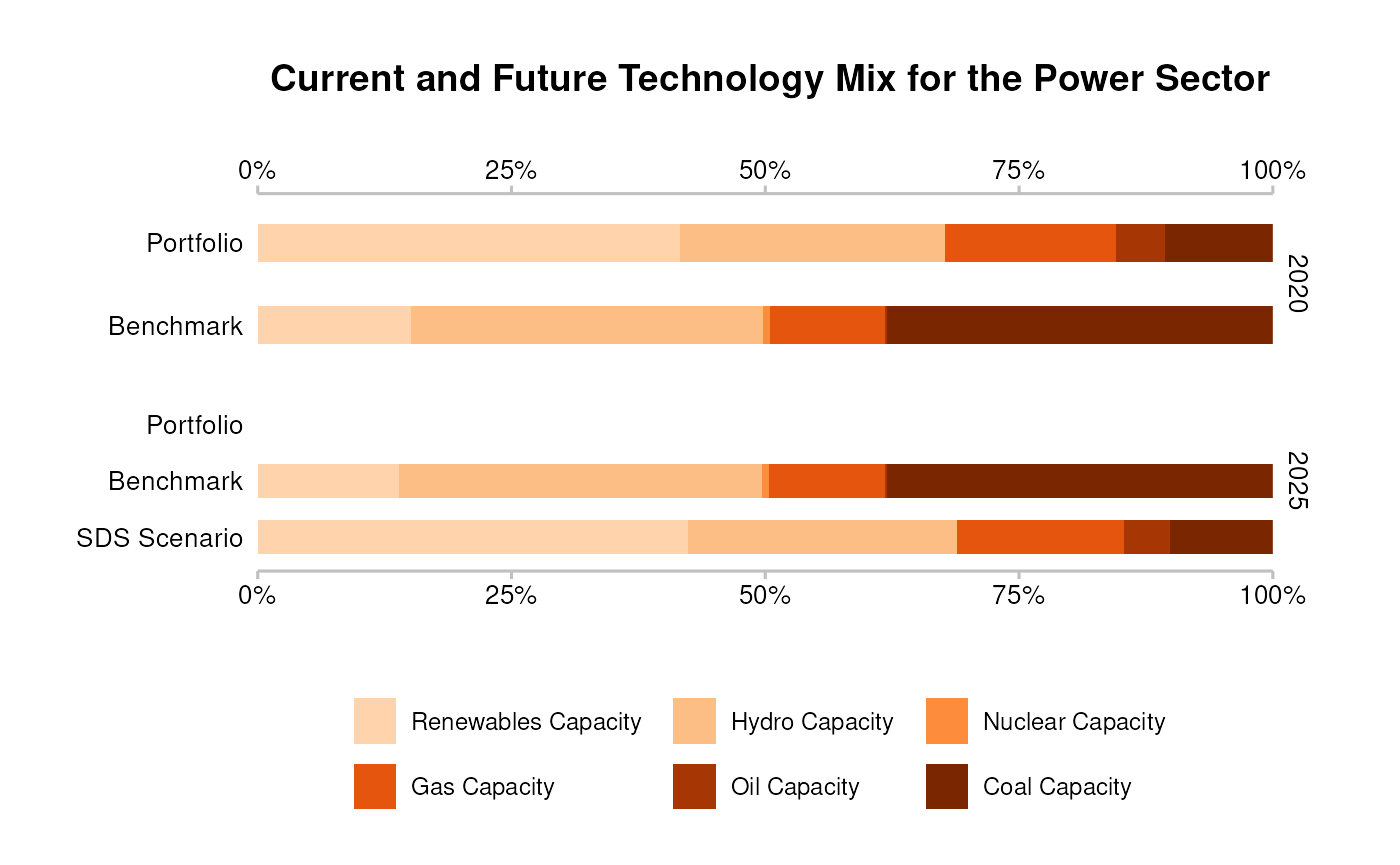
To obtain the technology mix chart for an individual company in your portfolio, you can run the following code (notice that we do not actually run the code here, as the output plot will look structurally almost the same as the tech mix plot for a portfolio):
# Pick the targets you want to plot.
data_company <- filter(
market_share_targets_company,
# provide the name of the company and "corporate_economy" to select the relevant emission intensity pathways
name_abcd %in% c("Mariani-Mariani s.r.l.", "corporate_economy"),
scenario_source == "demo_2020",
sector == "power",
region == "global",
metric %in% c("projected", "corporate_economy", "target_sds")
)
# Plot the technology mix
qplot_techmix(data_company) +
# Add labels to the bars. This is optional.
ggrepel::geom_label_repel(
aes(label = paste0(round(technology_share, 3) * 100, "%")),
min.segment.length = 0,
position = position_stack(vjust = 0.5),
show.legend = FALSE
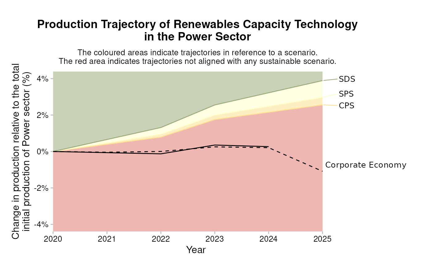
)Market Share: Technology-level volume trajectory
You can also plot the technology-specific volume trend. All starting values are normalized to 1, to emphasize that we are comparing the rates of build-out and/or retirement.
data_portfolio <- filter(
  market_share_targets_portfolio,
  sector == "power",
  technology == "renewablescap",
  region == "global",
  scenario_source == "demo_2020"
)

# to optionally display the emission factor metric at the end of the lines,
# we have to create an auxiliary data set
data_ends <- data_portfolio %>%
  dplyr::filter(year == min(.data$year) + 5) %>%
  dplyr::rename(value = "percentage_of_initial_production_by_scope")

qplot_trajectory(data_portfolio) +
  # Add labels to the end of the lines. This is optional.
  ggrepel::geom_text_repel(
    aes(label = paste0(round(value, 3) * 100, "%")),
    data = data_ends
  )
Again, the volume trajectory chart for an individual company in your portfolio can be obtained by running the following code (notice that we do not actually run the code here, as the output plot will look structurally almost the same as the volume trajectory plot for a portfolio):
data_company <- filter(
market_share_targets_company,
# provide the name of the company and "corporate_economy" to select the relevant emission intensity pathways
name_abcd %in% c("Mariani-Mariani s.r.l.", "corporate_economy"),
sector == "power",
technology == "renewablescap",
region == "global",
scenario_source == "demo_2020"
)
# to optionally display the emission factor metric at the end of the lines,
# we have to create an auxiliary data set
data_ends <- data_company %>%
dplyr::filter(year == min(.data$year) + 5) %>%
dplyr::rename(value = "percentage_of_initial_production_by_scope")
qplot_trajectory(data_company) +
# Add labels to the end of the lines. This is optional.
ggrepel::geom_text_repel(
aes(label = paste0(round(value, 3) * 100, "%")),
data = data_ends
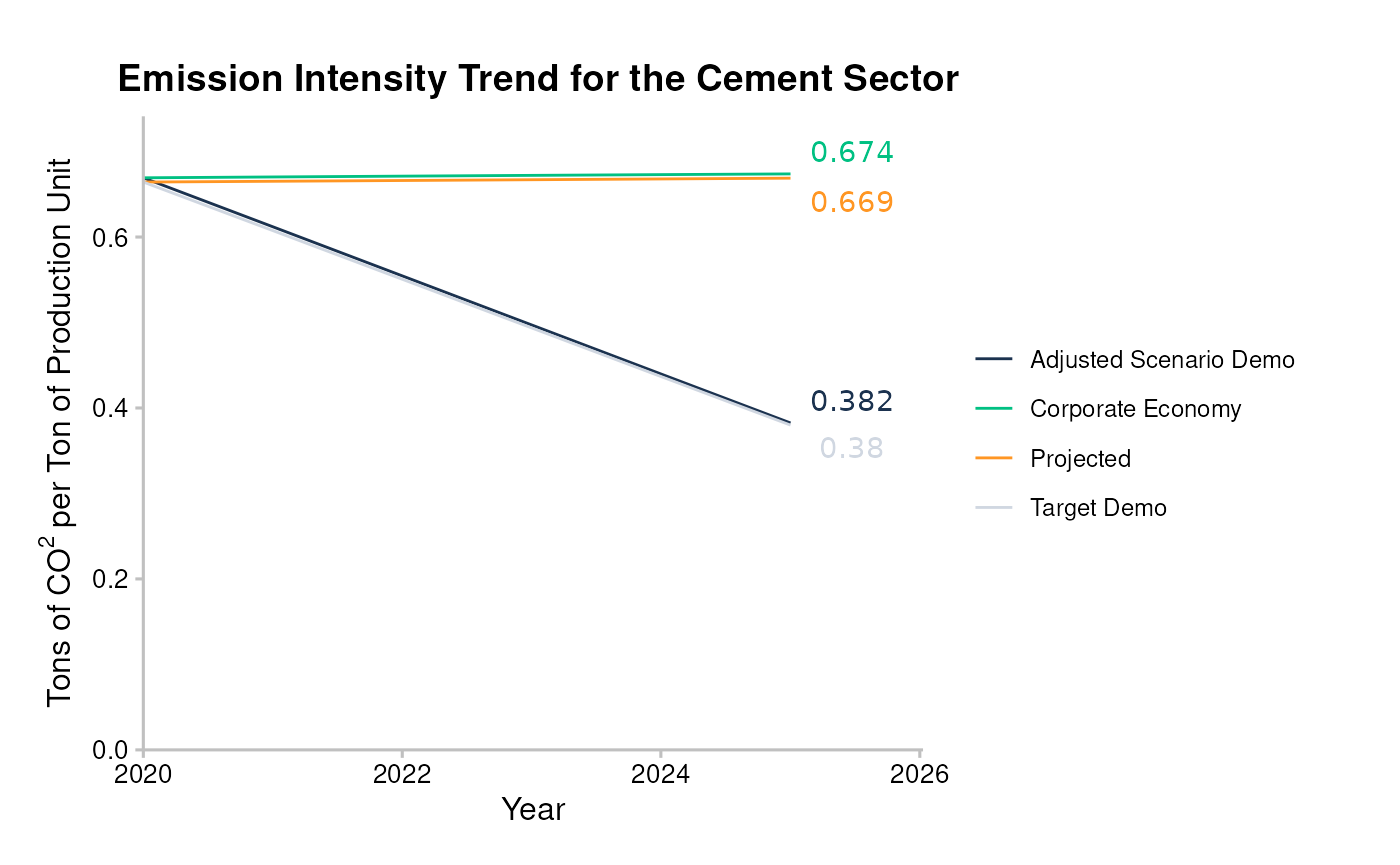
)SDA Target: Sector-level emission intensity
From the SDA output, we can compare the projected average emission intensity attributed to the portfolio, with the actual emission intensity scenario, and the scenario compliant SDA pathway that the portfolio must follow to achieve the scenario ambition by 2050.
data_portfolio <- filter(
  sda_targets_portfolio,
  sector == "cement",
  region == "global"
)

data_ends <- data_portfolio %>%
  dplyr::filter(year == min(.data$year) + 5) %>%
  dplyr::mutate(
    year = as.Date(strptime(as.character(year), "%Y")),
    label = pacta.loanbook::to_title(emission_factor_metric)
  )

qplot_emission_intensity(data_portfolio) +
  # Add labels to the end of the lines. This is optional.
  ggrepel::geom_text_repel(
    aes(label = round(emission_factor_value, 3)),
    data = data_ends,
    show.legend = FALSE
  )
The emission intensity plot can also be plotted for an individual company. Similarly to the above cases, you can create the company-level emissions intensity plot by running the following code (notice that we do not actually run the code here, as the output plot will look structurally almost the same as the emission intensity plot for a portfolio):
data_company <- filter(
  sda_targets_company,
  # provide the name of the company and "market" to select the relevant emission intensity pathways
  name_abcd %in% c("Kramer GmbH & Co. OHG", "market"),
  sector == "cement",
  region == "global"
)

# to optionally display the emission factor metric at the end of the lines, we have to create an auxiliary data set
data_ends <- data_company %>%
  dplyr::filter(year == min(.data$year) + 5) %>%
  dplyr::mutate(
    year = as.Date(strptime(as.character(year), "%Y")),
    label = pacta.loanbook::to_title(emission_factor_metric)
  )

qplot_emission_intensity(data_company) +
  # Add labels to the end of the lines. This is optional.
  ggrepel::geom_text_repel(
    aes(label = round(emission_factor_value, 3)),
    data = data_ends,
    show.legend = FALSE
  )
Exporting plots to an image file
All of the functions from pacta.loanbook that produce
plots, e.g. qplot_techmix() and
plot_trajectory(), return a ggplot object,
which can be saved as an image file using the
ggplot2::ggsave() function, for example:
emission_intensity_plot <- qplot_emission_intensity(data_portfolio)

ggplot2::ggsave(
  filename = file.path(tempdir(), "emission_intensity_plot.png"),
  plot = emission_intensity_plot
)
#> Saving 7.29 x 4.51 in image
Further customization of the image file characteristics can be
tweaked using the arguments of ggplot2::ggsave(),
e.g. device (filetype), width,
height, and dpi (resolution). See the
ggplot2::ggsave() documentation for more detail about the
options available.
PREVIOUS CHAPTER: Preparatory Steps
NEXT CHAPTER: Interpretation of Results