Custom 2DII colour and fill scales
scale_colour_2dii.RdA custom discrete colour and fill scales with colours from 2DII palettes.
Arguments
- palette
String with the name of the colour scale to be used. If not specified then the general 2dii scale is used
- colour_groups
A vector containing groups variable to which colours are assigned. It is needed when the data assigned to
colouraesthetic are not all contained in colour aliases of the palette.- ...
Other parameters passed on to
ggplot2::discrete_scale().
Examples
library(ggplot2, warn.conflicts = FALSE)
library(r2dii.plot, warn.conflicts = FALSE)
library(dplyr, warn.conflicts = FALSE)
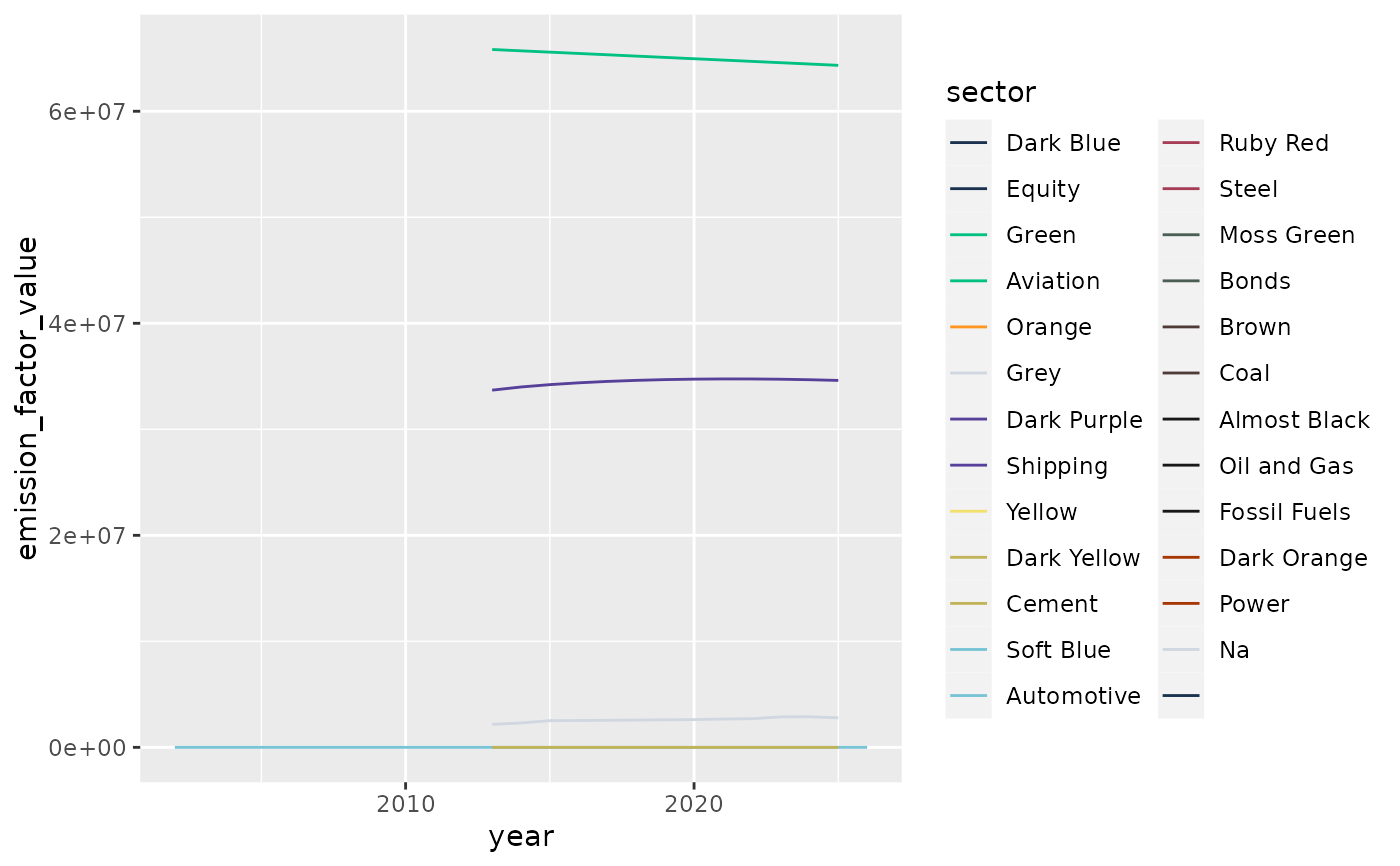
sda %>% filter(emission_factor_metric == "projected") %>%
ggplot() +
geom_line(aes(x = year, y = emission_factor_value, colour = sector)) +
scale_colour_2dii()
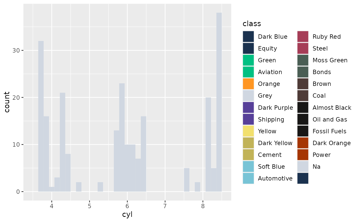
 mpg %>%
ggplot() +
geom_histogram(aes(cyl, fill = class), position = "dodge", bins = 5) +
scale_fill_2dii()
mpg %>%
ggplot() +
geom_histogram(aes(cyl, fill = class), position = "dodge", bins = 5) +
scale_fill_2dii()
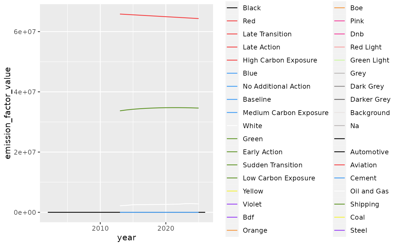
 sda %>% filter(emission_factor_metric == "projected") %>%
ggplot() +
geom_line(aes(x = year, y = emission_factor_value, colour = sector)) +
scale_colour_2dii(palette = "1in1000", colour_groups = sda$sector)
#> Assigning colours to unrecognised names in data: automotive, aviation, cement, oil and gas, shipping, coal, steel.
sda %>% filter(emission_factor_metric == "projected") %>%
ggplot() +
geom_line(aes(x = year, y = emission_factor_value, colour = sector)) +
scale_colour_2dii(palette = "1in1000", colour_groups = sda$sector)
#> Assigning colours to unrecognised names in data: automotive, aviation, cement, oil and gas, shipping, coal, steel.
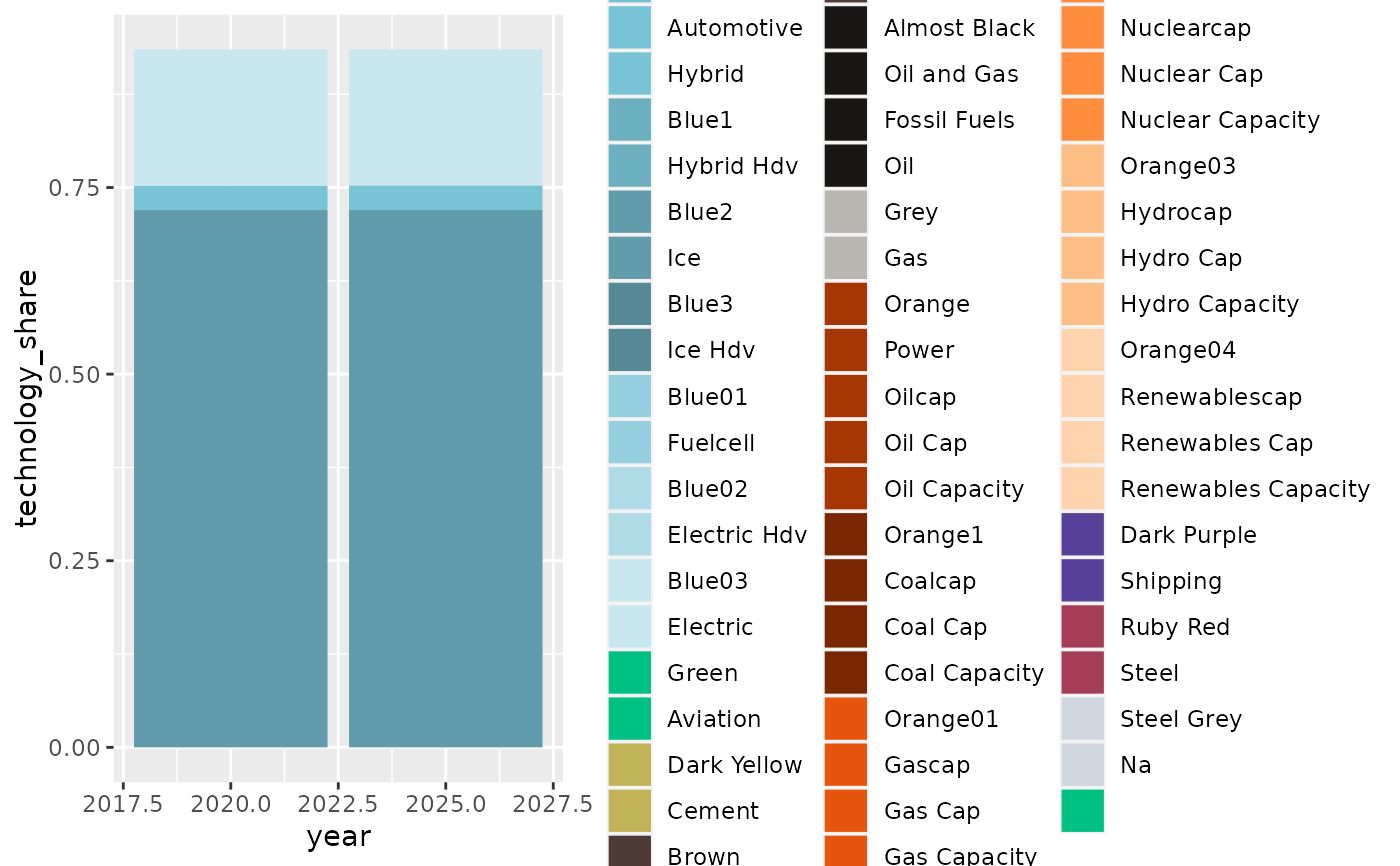
 market_share %>%
filter(sector == "automotive", year %in% c(2020, 2025), metric == "projected") %>%
ggplot() +
geom_bar(
stat = "identity",
aes(x = year, y = technology_share, fill = technology)) +
scale_fill_2dii(palette = "pacta")
market_share %>%
filter(sector == "automotive", year %in% c(2020, 2025), metric == "projected") %>%
ggplot() +
geom_bar(
stat = "identity",
aes(x = year, y = technology_share, fill = technology)) +
scale_fill_2dii(palette = "pacta")